Basic Example
This IPython notebook shows some common use cases.
First, import the most important modules:
import numpy as np
import matplotlib.pyplot as plt
from postcactus.simdir import SimDir
from postcactus import visualize as viz
from postcactus import grid_data as gd
Next, get a representation of a simulation directory:
sd = SimDir("/home/wkastaun/mydata1/results/BNS/SHT/bns_sht_mb1.51_d45_s1")
Get some simulation parameters (try tab-completion!) from the parfile:
xm = float(sd.initial_params.coordbase.xmax)
dx = float(sd.initial_params.coordbase.dx)
xm/dx
100.0
print sd.initial_params.reflectionsymmetry
reflectionsymmetry::avoid_origin_x       = "no"
reflectionsymmetry::avoid_origin_y       = "no"
reflectionsymmetry::avoid_origin_z       = "no"
reflectionsymmetry::reflection_x         = "no"
reflectionsymmetry::reflection_y         = "no"
reflectionsymmetry::reflection_z         = "yes"
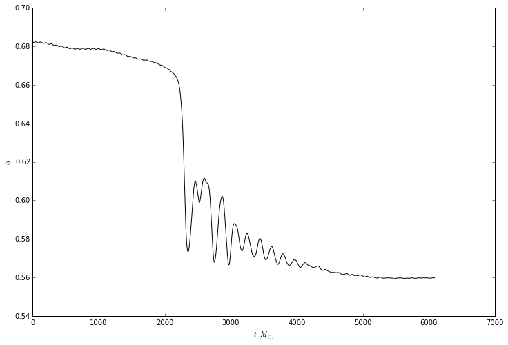
Get scalar data. Restarts will by merged transparently.
min_alp = sd.ts.min['alp']
Other norms are accessed the same way (try sd.ts.+TAB-KEY). For interactive work, there is a tab-completable list of available norms available as follows:
max_rho = sd.ts.max.fields.rho
Plot resulting timeseries using matplotlib.
plt.plot(min_alp.t, min_alp.y, 'k-');
plt.ylabel(r'$\alpha$');
plt.xlabel(r'$t \,[M_\odot]$');
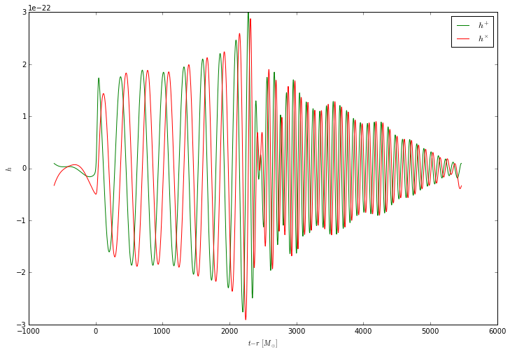
Graviational wave data from Psi4:
print sd.gwpsi4mp.available_dist
dist  = sd.gwpsi4mp.outermost
ffi_cut = 0.0155
hp,hc = sd.gwpsi4mp.get_strain(2, 2, dist, ffi_cut);
[50.0, 75.0, 100.0, 150.0, 200.0, 300.0, 400.0, 620.0]
mPC = 2.089553590485019e+19
plt.plot(hp.t-dist, hp.y / (100*mPC), 'g-', label=r'$h^+$');
plt.plot(hc.t-dist, hc.y / (100*mPC), 'r-', label=r'$h^\times$');
plt.xlabel(r'$t-r \,[M_\odot]$');
plt.ylabel(r'$h$');
plt.legend();
Grid data can be obtained in two ways: resampled to uniform grid while loading, or as a collection of components.
g = gd.RegGeom([180,180], [-40,-40], x1=[40,40]);
it = 4096
rho = sd.grid.xy.read('rho', it, geom=g, order=1);
Grid data is returned as a wrapper around numpy arrays which also knows the geometry. As for scalar data, sd.grid.xy.fields provides tab-completion of available data. Unless adjust_spacing=False is specified, the returned grid spacing will be adjusted to the next finer level:
print rho.data.shape
print rho.x0(), rho.x1(), rho.dx()
(201, 201)
[-40. -40.] [ 40.  40.] [ 0.4  0.4]
Binary arithmetic operations work as usual, unary operations are defined as methods.
rho_si = 6.176269145886163e+20 * rho
lgrho_cgs = rho_si.log10()
print lgrho_cgs.max()
17.6317886801
To obtain an array with the refinement level from which each point is read, use:
rlvl = sd.grid.xy.read('rho', it, geom=g, order=1, level_fill=True);
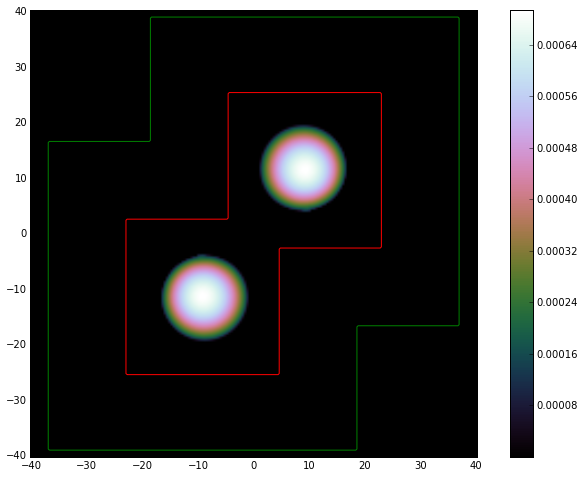
There are functions to plot 2D data as contour or color plot.
cm     = viz.get_color_map('cubehelix');
viz.plot_color(rho, bar=True, cmap=cm, interpolation='bilinear');
lvl    = -0.5+np.arange(3,6);
clrs   = ['y','g','r'];
viz.plot_contour(rlvl, levels=lvl, colors=clrs);
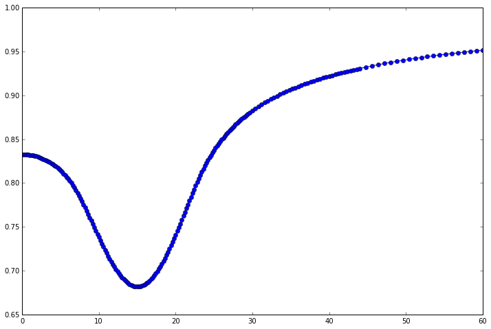
Reading 1D, 2D, and 3D grid data works in the same way. Note if data of the requested dimension is not available, the code automatically makes a cut of higher-dimensional data, if available. For 1D data, there is a special method that merges a hirachy into an irregularly spaced dataset using the finest available points.
alp_x = sd.grid.x.read('alp', 0);
x,alpx = gd.merge_comp_data_1d(alp_x);
plt.plot(x,alpx, 'bo-');
plt.xlim(0,60);
Apparent horizon data from AHFinderDirect, QuasiLocalMeasures, and (deprecated) IsolatedHorizons thorns is accessible as well:
sd2 = SimDir("/home/wkastaun/mydata2/results/aei/BNS/LS220/mb1.5_d50/spinf1_z4_nopi")
print sd2.ahoriz
Apparent horizons found: 2

--- Horizon 1 ---


Apparent horizon 1
  times (7.814400e+03..9.054720e+03)
  iterations (260480..301824)
  final state
    irreducible mass  = 2.439972e+00
    mean radius       = 2.426214e+00
    circ. radius xy   = 3.327424e+01
    circ. radius xz   = 2.947053e+01
    circ. radius yz   = 2.947057e+01

Spherical surface 0
  final state:
    M             = 2.647901e+00  (from QLM)
    M             = 2.647909e+00  (from IH)
    J/M^2         = 7.158759e-01  (from QLM)
    J/M^2         = 7.158779e-01  (from IH)
    J^i           = (6.374859e-14, 3.138668e-14, 5.022310e+00)  (from QLM)
    J^i           = (-2.633787e-08, -4.801370e-09, 5.022327e+00)  (from IH)
    r_circ_xy     = 3.327421e+01  (from QLM)
    r_circ_xy     = 3.327409e+01  (from IH)
    r_circ_xz     = 2.947098e+01  (from QLM)
    r_circ_xz     = 2.947445e+01  (from IH)
    r_circ_yz     = 2.947539e+01  (from QLM)
    r_circ_yz     = 2.947373e+01  (from IH)

  Shape available: True

--- Horizon 2 ---


Apparent horizon 2
  times (7.814400e+03..9.054720e+03)
  iterations (260480..301824)
  final state
    irreducible mass  = 2.439972e+00
    mean radius       = 2.426214e+00
    circ. radius xy   = 3.327424e+01
    circ. radius xz   = 2.947053e+01
    circ. radius yz   = 2.947057e+01

Spherical surface 1
  final state:
    M             = 2.647901e+00  (from QLM)
    M             = 2.647909e+00  (from IH)
    J/M^2         = 7.158759e-01  (from QLM)
    J/M^2         = 7.158779e-01  (from IH)
    J^i           = (-6.404892e-14, -3.137923e-14, 5.022310e+00)  (from QLM)
    J^i           = (-2.633792e-08, -4.801398e-09, 5.022327e+00)  (from IH)
    r_circ_xy     = 3.327421e+01  (from QLM)
    r_circ_xy     = 3.327409e+01  (from IH)
    r_circ_xz     = 2.947098e+01  (from QLM)
    r_circ_xz     = 2.947445e+01  (from IH)
    r_circ_yz     = 2.947539e+01  (from QLM)
    r_circ_yz     = 2.947373e+01  (from IH)

  Shape available: True
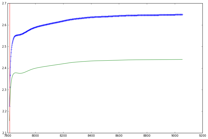
ah   = sd2.ahoriz.largest
m_ah = ah.ih.M
mirr_ah = ah.ih.M_irr
plt.plot(m_ah.t, m_ah.y, 'b-+')
plt.plot(mirr_ah.t, mirr_ah.y, 'g-')
plt.axvline(x=ah.tformation, color='r');